Basics of Pandas

Pandas is a Python library used for data analysis and data manipulation. We'll use pandas to explore the data of many different biological datasets. Pandas is a very extensive package with many complex functions, but these notes will cover basic, introductory information on pandas.

Overview of Pandas DataFrames

In pandas, we can create DataFrames with our data. DataFrames are 2-dimensional labeled data structures, consisting of rows and columns filled with data. In most pandas DataFrames, the rows are labeled by an index, starting a index 0, while the columns are labeled by a name of choice. Each column contains data, which can be of any Python data type, like an integer or string.

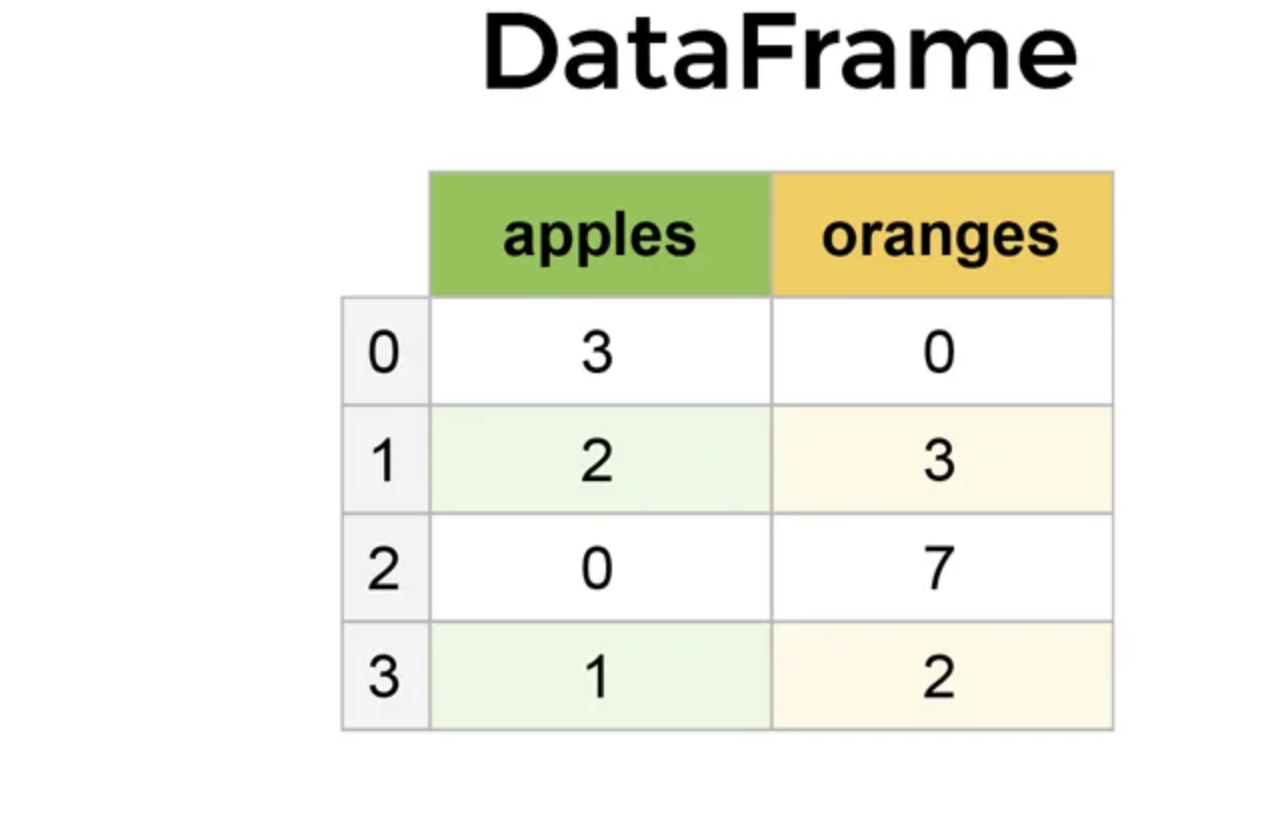
Below is an example of a pandas DataFrame. The rows are indexed starting at 0 and going to 3. The column names are "apples" and "oranges". The data in each column are integers.

Creating a DataFrame

Pandas DataFrames can be created in various ways, like manually creating the DataFrame or reading in different files to create DataFrames with. We often create our DataFrames with csv files, which stands for comma-separated values, as the data in the file is separated by commas.

In pandas, the function read_csv() can be used to read in data and create a pandas DataFrame. Let's try it with the surveys.csv file, which contains data on various species that have been recorded between 1977 and 2002. The dataset includes a record id, the month, day, and year when the specimen was recorded, a plot id and species id, and the sex, hindfoot length, and weight of the specimen.

# Importing packages
import pandas as pd
import numpy as np

# Reads in the species data
df = pd.read_csv('surveys.csv')
df

	record_id	month	day	year	plot_id	species_id	sex	hindfoot_length	weight
0	1	7	16	1977	2	NL	M	32.0	NaN
1	2	7	16	1977	3	NL	M	33.0	NaN
2	3	7	16	1977	2	DM	F	37.0	NaN
3	4	7	16	1977	7	DM	M	36.0	NaN
4	5	7	16	1977	3	DM	M	35.0	NaN
...	...	...	...	...	...	...	...	...	...
35544	35545	12	31	2002	15	AH	NaN	NaN	NaN
35545	35546	12	31	2002	15	AH	NaN	NaN	NaN
35546	35547	12	31	2002	10	RM	F	15.0	14.0
35547	35548	12	31	2002	7	DO	M	36.0	51.0
35548	35549	12	31	2002	5	NaN	NaN	NaN	NaN

35549 rows × 9 columns

We can confirm that df is indeed a DataFrame by using the type() function.

type(df)

pandas.core.frame.DataFrame

Yep, that's a pandas DataFrame!

Viewing DataFrame Information

There are a few ways to view the data in a pandas DataFrame. head() allows you to view the first few rows of the DataFrame, while tail() allows you to view the last rows. You can also select the number of rows you want to view by passing the integer of row numbers as an argument to the function.

# Views the first rows of the DataFrame
df.head()

	record_id	month	day	year	plot_id	species_id	sex	hindfoot_length	weight
0	1	7	16	1977	2	NL	M	32.0	NaN
1	2	7	16	1977	3	NL	M	33.0	NaN
2	3	7	16	1977	2	DM	F	37.0	NaN
3	4	7	16	1977	7	DM	M	36.0	NaN
4	5	7	16	1977	3	DM	M	35.0	NaN

# Views the last 3 rows of the DataFrame
df.tail(3)

	record_id	month	day	year	plot_id	species_id	sex	hindfoot_length	weight
35546	35547	12	31	2002	10	RM	F	15.0	14.0
35547	35548	12	31	2002	7	DO	M	36.0	51.0
35548	35549	12	31	2002	5	NaN	NaN	NaN	NaN

We can also view the number of rows and columns in the DataFrame using the shape attribute. Attributes are properties of a DataFrame that can be fetched to provide information on the DataFrame. The attribute outputs two values, with the first being the numbers of rows and the second being the number of columns.

# Views the shape of the DataFrame
df.shape

(35549, 9)

Our DataFrame has 35549 rows and 9 columns.

Working with Columns in DataFrames

We can individually view the columns of a DataFrame with the columns attribute.

# Views the columns of a DataFrame
df.columns

Index(['record_id', 'month', 'day', 'year', 'plot_id', 'species_id', 'sex',
       'hindfoot_length', 'weight'],
      dtype='object')

We can also select a column to view in a pandas DataFrame. The basic syntax for this is df["column name"].

# Selects and views the species_id column
df['species_id']

0         NL
1         NL
2         DM
3         DM
4         DM
        ... 
35544     AH
35545     AH
35546     RM
35547     DO
35548    NaN
Name: species_id, Length: 35549, dtype: object

The selected column is a pandas Series, which we can see by using the type() function. A Series is a labeled array, and it retains the row indexing from the DataFrame.

# Views the type of a selected column
type(df['hindfoot_length'])

pandas.core.series.Series

If we want to get the values of the columns as an array, rather than a Series, we can use the values attribute.

# Gets the values of the hindfoot length column as an array
df['hindfoot_length'].values

array([32., 33., 37., ..., 15., 36., nan], shape=(35549,))

Basic analyses can be done on individual columns, like calculating the mean or maximum value.

# Calculates the mean hindfoot length
np.mean(df['hindfoot_length'])

np.float64(29.287931802277498)

# Calculates the maximum hindfoot length
np.max(df['hindfoot_length'])

np.float64(70.0)

Manipulating DataFrames

A new DataFrame can be created by selecting specific columns from another DataFrame. This is similar to selecting a single column, but you instead include a list of columns to subset and turn into a new DataFrame. We'll include the copy() code to prevent any warnings.

# Creates a new DataFrame with the hindfoot length and weight columns
length_weight_df = df[['hindfoot_length','weight']].copy()
length_weight_df

	hindfoot_length	weight
0	32.0	NaN
1	33.0	NaN
2	37.0	NaN
3	36.0	NaN
4	35.0	NaN
...	...	...
35544	NaN	NaN
35545	NaN	NaN
35546	15.0	14.0
35547	36.0	51.0
35548	NaN	NaN

35549 rows × 2 columns

New columns can be added to a DataFrame. This can be done with the code df["new column name"] = column data.

If you include an array or list of the same length as the number of rows, then each DataFrame row will contain the data from the corresponding entry in the array or list. If you include one value for the column data, then every entry for the column will contain that value.

# Adds a column with a sequence from 0 to 35548
length_weight_df['sequence'] = np.arange(df.shape[0])
# Adds a column with the word "Nature"
length_weight_df['word'] = 'Nature'
length_weight_df

	hindfoot_length	weight	sequence	word
0	32.0	NaN	0	Nature
1	33.0	NaN	1	Nature
2	37.0	NaN	2	Nature
3	36.0	NaN	3	Nature
4	35.0	NaN	4	Nature
...	...	...	...	...
35544	NaN	NaN	35544	Nature
35545	NaN	NaN	35545	Nature
35546	15.0	14.0	35546	Nature
35547	36.0	51.0	35547	Nature
35548	NaN	NaN	35548	Nature

35549 rows × 4 columns

Conditional statements can be used to select data that meets a specific condition. The basic syntax for this is df[df["column name"] {conditional operator} {condition}]. Below are some examples of subsetting using conditionals.

# Subsets rows with the DM species
df[df['species_id'] == "DM"]

	record_id	month	day	year	plot_id	species_id	sex	hindfoot_length	weight
2	3	7	16	1977	2	DM	F	37.0	NaN
3	4	7	16	1977	7	DM	M	36.0	NaN
4	5	7	16	1977	3	DM	M	35.0	NaN
7	8	7	16	1977	1	DM	M	37.0	NaN
8	9	7	16	1977	1	DM	F	34.0	NaN
...	...	...	...	...	...	...	...	...	...
35532	35533	12	31	2002	14	DM	F	36.0	48.0
35533	35534	12	31	2002	14	DM	M	37.0	56.0
35534	35535	12	31	2002	14	DM	M	37.0	53.0
35535	35536	12	31	2002	14	DM	F	35.0	42.0
35536	35537	12	31	2002	14	DM	F	36.0	46.0

10596 rows × 9 columns

# Subsets rows that are greater than the year 1990
df[df["year"] > 1990]

	record_id	month	day	year	plot_id	species_id	sex	hindfoot_length	weight
18189	18190	1	11	1991	7	RM	F	17.0	11.0
18190	18191	1	11	1991	12	OL	M	21.0	31.0
18191	18192	1	11	1991	17	RM	F	16.0	9.0
18192	18193	1	11	1991	2	DM	F	34.0	48.0
18193	18194	1	11	1991	12	DO	F	36.0	36.0
...	...	...	...	...	...	...	...	...	...
35544	35545	12	31	2002	15	AH	NaN	NaN	NaN
35545	35546	12	31	2002	15	AH	NaN	NaN	NaN
35546	35547	12	31	2002	10	RM	F	15.0	14.0
35547	35548	12	31	2002	7	DO	M	36.0	51.0
35548	35549	12	31	2002	5	NaN	NaN	NaN	NaN

17360 rows × 9 columns